Long-Term Imaging of Identified Neural Populations using Microprisms in Freely Moving and Head-Fixed Animals

Summary

When integrated with a head-plate and an optical design compatible with both single- and two-photon microscopes, the microprism lens presents a significant advantage in measuring neural responses in a vertical column under diverse conditions, including well-controlled experiments in head-fixed states or natural behavioral tasks in freely moving animals.

Abstract

With the advancement of multi-photon microscopy and molecular technologies, fluorescence imaging is rapidly growing to become a powerful approach for studying the structure, function, and plasticity of living brain tissues. In comparison to conventional electrophysiology, fluorescence microscopy can capture the neural activity as well as the morphology of the cells, enabling long-term recordings of the identified neuron populations at single-cell or subcellular resolution. However, high-resolution imaging typically requires a stable, head-fixed setup that restricts the movement of the animal, and the preparation of a flat surface of transparent glass allows visualization of neurons at one or more horizontal planes but is limited in studying the vertical processes running across different depths. Here, we describe a procedure to combine a head plate fixation and a microprism that gives multilayer and multimodal imaging. This surgical preparation not only gives access to the entire column of the mouse visual cortex but allows two-photon imaging in a head-fixed position and one-photon imaging in a freely moving paradigm. Using this approach, one can sample identified cell populations across different cortical layers, register their responses under head-fixed and freely moving states, and track the long-term changes over months. Thus, this method provides a comprehensive assay of the microcircuits, enabling direct comparison of neural activities evoked by well-controlled stimuli and under a natural behavioral paradigm.

Introduction

The advent of in vivo two-photon fluorescent imaging^1,2, combining the new technologies in optical systems and genetically modified fluorescence indicators, has emerged as a powerful technique in neuroscience to investigate the intricate structure, function, and plasticity in the living brain^3,4. In particular, this imaging modality offers an unparalleled advantage over traditional electrophysiology by capturing both the morphology and dynamic activities of neurons, thereby facilitating long-term tracking of identified neurons^5,6,7,8.

Despite its noteworthy strengths, the application of high-resolution fluorescence imaging often necessitates a static, head-fixed setup that constrains the animal's mobility^9,10,11. Additionally, the use of a transparent glass surface for visualizing neurons restricts observations to one or more horizontal planes, limiting the exploration of the dynamics of vertical processes that extend across different cortical depths¹².

Addressing these limitations, the present study outlines an innovative surgical procedure that integrates head plate fixation, microprism, and miniscope to create an imaging modality with multilayer and multimodal capabilities. The microprism allows the observation of the vertical processing along the cortical column^13,14,15,16, which is critical in understanding how information is processed and transformed as it moves through different layers of the cortex and how the vertical processing is altered during plastic changes. Moreover, it permits imaging of the same neural populations in a head-fixed paradigm and in a freely moving setting, encompassing the versatile experimental settings^17,18,19: for example, head-fixation is often required for well-controlled paradigms like sensory perception assessment and stable recordings under 2-photon paradigm, while freely moving offers a more natural, flexible environment for behavioral studies. Therefore, the ability to conduct a direct comparison in both modes is crucial to furthering our understanding of the microcircuits that enable flexible, functional responses.

In essence, the integration of head plate fixation, microprism, and miniscope in fluorescence imaging offers a promising platform for probing the intricacies of the brain's structure and functionality. Researchers can sample identified cell populations across various depths spanning all cortical layers, directly compare their responses in both well-controlled and natural paradigms, and monitor their long-term alterations over months²⁰. This approach offers valuable insight into how these neural populations interact and change over time under different experimental conditions, providing a window into the dynamic nature of neural circuits.

Protocol

All experiments were conducted according to the UK Animals (Scientific Procedures) Act 1986 under personal and project licenses approved and issued by the UK Home Office following appropriate ethics review. Adult transgenic lines CaMKII-TTA; GCaMP6S-TRE²¹ were bred and their offspring used in the experiment. For the safety of the experimenters and the maintenance of sterile conditions, all the procedures were performed under aseptic conditions and with full personal protective equipment.

1. Pre-operative preparation

1. To minimize edema, administer Dexamethasone (0.2 mg/kg) subcutaneously, 12-24 h before surgery.
2. Sterilize all surgical tools in an autoclave and sterilize the surgical area with stabilized hypochlorous acid with distilled water and 70% ethanol prior to surgery. Ensure all surgical equipment is turned ON.
3. Anaesthetize the animal (24 weeks old, male weighing 31 g) using isoflurane with an induction dose of 5%, which is decreased to 1%-2% once the mouse is on the stereotaxic frame, with O₂ kept between 1-2 L/min. Inject NSAIDs (Carprofen, 2.5 mg/kg) subcutaneously.
4. Check for absence of toe-pinch reflex to assess the depth of anesthesia (increase isoflurane concentration in 0.5% increments if reflex seen).
5. Shave the animal's head, using a trimmer, from behind the ears to slightly above the eyes. Clean this area with an alcohol wipe and povidone-iodine solution, ensuring to avoid contact with the animal's eyes.
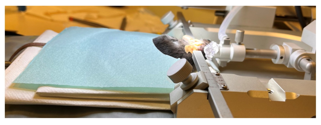
6. Mount the animal onto the homeothermic heating pad and stereotaxic frame fitted with ear and teeth bars and secure the head. Ensure the head is stable, as this is crucial for the following procedure to be successful (Figure 1).
7. Apply ophthalmic ointment over the animal's eyes to prevent them from drying during surgery and cover them with foil to protect them from light. Cover the animal with a sterile surgical cover.

Figure 1: Pre-operation preparation. The mouse is placed onto the stereotaxic frame, secured by a nose piece and ear bars. The mouse is placed on a temperature-regulated heated pad. Eyes have ophthalmic ointment on them and are covered by aluminum foil. The head is shaved, and the skull is exposed. A sterile cover is placed over the animal. Please click here to view a larger version of this figure.

2. Craniotomy

1. Using surgical scissors, incise the skin along the midline of the shaved area of the head to expose the skull.
2. Clean the skull using a sterile cotton swab and diluted hydrogen peroxide (3% w/v of 35% H₂O₂ in 97% dH₂O) for 1-3 s to remove any connective tissue (Figure 2A). Dry the skull using drop of 70% ethanol and a new sterile cotton swab.
3. Align the skull anteriorly/posteriorly (AP) and medially/laterally (ML) to ensure an accurate implantation site. To do this, measure the dorsoventral (DV) depth of the skull at both bregma and lambda and ensure that the difference between the two is <0.03 mm. For the mediolateral alignment, measure equidistant points on both parietal bones from the midline and again ensure the DV difference is <0.03 mm.
4. Using bregma as the origin, find and mark the desired cortical area; here, these are monocular primary visual cortex (V1), AP: -3.5 mm, ML: -2.5 mm.
5. Use a trephine drill bit (1.8 mm diameter) and dental drill (10,000 rpm speed) to expose the cortex, ensuring the mark for the desired cortical area (monocular V1) is located within the bottom third of the drill-bit window. 
   1. Ensure the angle of the drill bit is perpendicular to the curvature of the skull. This will ensure an even craniotomy and will prevent damage to the dura or cortex.
   2. Drill until there is a decrease in resistance and then stop (Figure 2B). Carefully remove the detached bone fragment using a 23G needle tip (Figure 2C).
   3. Clean the exposed cortex with surgical foam saturated in cold artificial cerebrospinal fluid (ACSF) to remove any debris and stop any bleeding that may occur.
   4. Always keep the exposed cortex hydrated, using cold ACSF, throughout the surgery.

Figure 2: Craniotomy. (A) Skin incision between bregma and lambda is shown. Connective tissue has been removed from the exposed surface. (B) Craniotomy by trephine drill before removal of the bone fragment. (C) Craniotomy after removal of bone fragment, showing intact dura and cortex (scale bar represents 0.5 mm). Please click here to view a larger version of this figure.

3. Pre-cut incision

NOTE: To be considered when performing the precut incision, the incision and microprism implantation will need to be anterior to the imaging region of interest (ROI). This is to allow a full and accurate field of view. In the context of this protocol, the incision will be performed along the mediolateral axis, and the microprism is orientated facing the posterior (Figure 3B).

1. To help with the insertion and to alleviate pressure in the cortex during the insertion of the microprism, make an incision.
2. Attach the surgical knife to the stereotaxic arm holder and orientate the blade or stereotaxic arm so that it will cut along the ML axis.
3. Move the knife to the desired AP coordinate (AP: -3.4mm); the prism is required to be in front of the ROI, so make the incision 100 µm anterior of the imaging ROI AP coordinate (-3.5mm).
4. Now moving the knife to the medial edge of the craniotomy, where it meets the skull, slowly lower the knife until it reaches the bone and then stop. As the bone thickness is 200 µm, incorporate this value into the total insertion depth (see step 5.1 calculation).
5. Optimal imaging is at the center of the prism i.e., 500 µm; therefore, ensure this depth aligns with the cortical column depth (ROI DV: - 0.35 mm).
   1. Incorporating the thickness of the skull into the calculation of depth, use the equation below, which determines how deep the pre-cut incision needs to be from the surface of the skull. For this protocol, the depth of implantation is calculated as:
      Bone thickness (200 µm) + imaging ROI (e.g., 350 µm) + remaining microprism depth (500 µm) = 1,050 µm
6. Ensure the length of the incision is more than 1 mm but not excessive; therefore, a distance of 1.2 mm is ideal, with the monocular ML coordinate being in the middle of this distance.
7. When ready to perform the incision, remove excess ACSF so that vision is not obscured (Figure 3A).
   1. Move the knife from the medial edge of the craniotomy to the starting medial coordinate of the incision. Slowly (10 µm/s) lower down the knife into the cortex.
   2. Once the dura is pierced and the knife has entered the cortex, apply a drop of cold ACSF onto the cortex to keep the tissue lubricated and hydrated during the incision.
8. Once the final depth has been reached, begin moving the knife along the ML axis (at a rate of 10 µm/s).
   1. Keep observing the surrounding tissue as the incision is being made. If the tissue is dragging along with the knife, move the knife up and down a few times to ensure the tissue is being cut, and then continue along laterally, remembering to put the knife back to its final depth.
9. When complete, slowly raise the knife. If blood emerges during the incision, use this time to clean the incision site with ACSF-soaked surgical foam to dilute the blood and push any blood within the incision out. Remember to leave a fresh, saturated surgical foam over the exposed cortex until ready to insert the microprism.

Figure 3: Microprism implantation. (A) Pre-cut incision. (B) Schematic of the integrated microprism lens demonstrating its position within the cortex (C) Integrated microprism lens in the correct orientation to pre-cut incision before insertion into the cortex (scale bar represents 0.5 mm). (D) Example of cement build-up around the integrated lens to secure its attachment to the skull. Please click here to view a larger version of this figure.

4. Microprism insertion and head plate implantation

1. The microprism lens is composed of a gradient index lens attached to a prism at the distal end of the lens, which is integrated into a baseplate. Attach the microprism to the implant kit.
2. Ensure the imaging side of the prism is opposite to the baseplate screw. To help with the insertion and placement of the microprism, attach it to the stereotaxic frame and orient the prism so that it aligns with the incision (Figure 3C).
3. Slowly lower the microprism into the incision site (10 µm/s). Remember to remove ACSF when initially inserting the prism, but once in the cortex, flush with cold ACSF to lubricate insertion.
   1. The cortex should remain stable while the prism is lowered into the incision; if not, add extra ACSF and agitate the cortex by moving the prism up and down to loosen the cortex from the prism.
4. Once the final depth has been reached, dry the exposed cortical surface using sterile tissue, being careful not to touch the prism.
5. Cover the exposed cortical area surrounding the prism, as well as the lens, with a protective layer of silicone adhesive, minimising excess adhesive on the surrounding skull and dummy scope.
6. Once cured (5-10 min), attach the headplate to the skull to stabilize the head during head-fixed imaging.
   1. Ensure the headplate is posterior enough so as not to interfere with the placement of the implant and to allow adequate application of cement to properly secure the implant.
   2. Ensure the midline of the headplate lies slightly right of implanted lens to ensure that both sides of the headplate can be secured to the head-stage when performing head-fixed experiments
7. Apply adhesive cement to the headplate and skull.
   1. Prepare adhesive dental cement by mixing 1 scoop of opaque cement powder with 4 drops of mixing medium and applying one drop of the catalyst.
   2. Place cement on both the headplate and skull and hold the headplate in place until cured, ensuring it’s parallel with the ear bars (through visual examination, inspect both from above and behind the animal’s head).
8. Apply adhesive cement to cover the rest of the exposed skull and tissue, incorporating the microprism (up to the base of the baseplate) and headplate.
9. Do not get cement on the baseplate, dummy microscope, or any of its components. Keep applying the adhesive cement until the microprism and headplate are covered and are stable (Figure 3D).
10. When the cement has cured, detach the dummy microscope by moving the stereotaxic arm upwards slowly while stabilizing the microprism with forceps (they are connected through magnets, therefore some resistance during the separation might be felt).
11. Insert the protective cover onto the lens and tighten the screw to secure it in place.
12. Remove the animal from the stereotaxic frame, allow it to recover in a warm recovery box, and administer warmed sterile 0.9% saline subcutaneously (3% of body weight).
13. Once the animal is awake and moving, place it back in a clean single-housed cage. Monitor the animal and administer additional post-surgery analgesia per the local institution’s policy on analgesia.
14. Wait for 4 weeks after surgery, the animal should be ready for imaging.

5. One-photon calcium imaging of cortical layers in freely moving mice

NOTE: It is essential to utilize images captured from the original imaging session each time to ensure accurate acquisition of the intended imaging plane. These identified landmarks, along with the neurons, play a critical role in the alignment process described in detail in step 9 of the protocol. When acquiring one-photon data, the miniscope is both the imaging system and the laser source. Excitation uses LED with a power range of 0-2 mW/mm² at the objective front surface. The laser uses an excitation wavelength of 455 ± 8nm (blue light) for GCaMP signaling. The lens focus slider can be used to adjust the focus (Z axis), which is represented on the interface as 0-1000, where 0 represents a 0µm working distance, and 1000 represents the maximum 300µm working distance.

1. Prior to acquiring data, let the animal acclimatize to the room and the open arena for 1 h before the recording session.
2. Before imaging, disinfect and clean everything with appropriate disinfectants (e.g., stabilized hypochlorous acid with distilled water and 70% ethanol).
3. Set up the DAQ box by connecting it to a computer and launching the data acquisition software. Establish a direct connection via an ethernet cable to minimize dropped frames; however, the wireless connection mode might suffice depending on the strength of the wireless connection.
4. Attach the miniscope to the animal's baseplate under a gentle scruff.
   1. First, remove the protective cover from the baseplate by unscrewing the set screw. Hold the cover by its aperture with forceps. Then, attach the miniscope to the baseplate, where the cover sits.
   2. Check the orientation of the miniscope in relation to the baseplate before installing it so that the side with the marking of the screw, faces the screw.
   3. Once the miniscope is attached, tighten the set screw to stabilize it. Only advance the set screw until some resistance can be felt. Overtightening the set screw would potentially damage the miniscope and should thus be avoided.
5. Connect the miniscope to the DAQ box and prepare the software for recording.
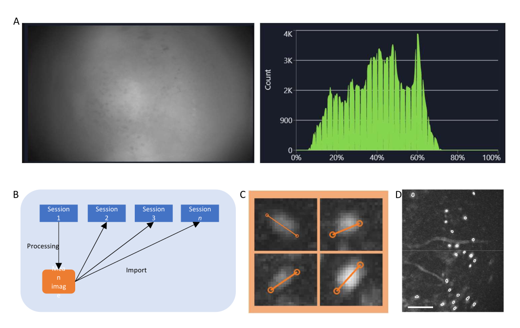
   1. In the data acquisition software, turn the stream on for the miniscope and adjust the recording parameters (imaging frame rate, gain, LED power, efocus value) to achieve a clear field of view (Figure 4A).
   2. Turn on the histogram window and adjust the gain and LED power so that the intensity recorded sits between 35% to 70% .
   3. If conducting a longitudinal study, refer to the recordings or snapshots taken in a previous session and adjust the efocus value so that the same imaging plane is clearly seen.
6. Start the experiment and data acquisition.
7. After the completion of the experiment, remove the animal from the behavioral apparatus.
   1. Under a gentle scruff, loosen the set screw and remove the miniscope from the animal's baseplate.
   2. Return the protective cover to the baseplate and stabilize it with the set screw.
8. Return the animal to its home cage (proceed to step 7 if wanting to process one-photon data).

Figure 4: Data acquisition and processing with software. (A) An image showing the real-time stream from the miniscope. It is recommended to adjust the lens focus value, so that a clear view is seen in the streaming window, along with the gain and the imaging laser power (B) Schematic graph illustrating the recommended alignment workflow for sessions recorded on different time points. It is recommended to generate a mean image from the first session, following the instructions for the data processing software. This image should be used as the reference image during motion correction for the following sessions. (C) Examples of four cells from the same max-projected ΔF/F image. An orange line is drawn across each cell to measure its cell diameter in pixels, the average of which is taken as an input argument for the cell identification algorithm (top left: 13, top right: 11, bottom left: 12, bottom right: 13). (D) Output of the cell identification algorithm after manual curation (image cropped). White outlines represent the identified cells (scale bar represents 100 µm). Please click here to view a larger version of this figure.

6. Two-photon calcium imaging of cortical layers in head-fixed mice

NOTE: For two-photon laser scanning microscopy, the light source is a tunable ultrafast laser with an excitation wavelength of 920 nm. Excitation power, measured at the objective, was typically between 100-150 mW and adjusted in each session to achieve similar levels of fluorescence. Emission light was filtered by an emission filter (525/70 nm) and measured by an independent photomultiplier tube (PMT), referred to as a green channel. Images were acquired with a 20x air immersion objective (NA = 0.45, 6.9-8.2 mm working distance).

1. Prior to acquiring data, habituate the animal to the apparatus in the days before (to make the animal become comfortable with the behavioral setup). Allow the animal to spend 15-30 min a day, for 2-3 days, exploring the setup or until they display naturalistic behavior before beginning the data acquisition.
2. Turn on the two-photon imaging system, launch acquisition software, and switch the laser ON. Make sure that the lasers are shuttered and PMTs are turned off before continuing.
3. Clean two-photon imaging apparatus with stabilized hypochlorous acid with distilled water and 70% ethanol.
4. Make sure to adjust the apparatus to fit the animal's size. Gently attach the mouse and its headplate to the head-stage setup and screw it in place to stabilize the mouse's head.
5. Once attached, remove the lens cover (refer to step 5.4.1), and align the objective so that it is over the baseplate.
6. Use the epifluorescence and XYZ stage controls to bring the cortical tissue into focus.
7. Once the cortical layers are visible, switch the microscope to allow two-photon imaging (swap out the mirror for the dichroic mirror, close the fluorescent shutter, and turn off the epifluorescence laser and monitor). Make sure to turn OFF the main lights so as to protect the PMTs when imaging.
8. Set up parameters to optimize acquired image files.
   1. Use resonant acquisition mode for calcium imaging as it can capture the rapid firing of GCaMP signals.
   2. Adjust laser power, PMT gain, zoom, and look-up tables (LUTs) to obtain an optimal image and refer to the one-photon image to ensure that the correct focal plane is being imaged.
   3. Begin imaging of cortical layers with the two-photon system with synchronized behavioral monitoring and stimulus inputs (if applicable).
   4. Make sure to save these acquisition parameters and XYZ distances if wanting to reproduce identical images over time.
9. To capture a z-stack of the cortical layers, follow the steps described below.
   1. Find the plane to start the z-stack from, adjust the acquisition parameters to optimize the image, and mark this as the starting point on the software.
   2. Next, using the Z control, move down the stack, only adjusting the laser power to maintain a constant luminance of the stack, and mark the end of the stack on the software.
   3. Critical step: using the Relative Exponential Gradient option under the Laser Power Gradient tab, allow the software to calculate the increase in laser power as it moves through the z-stack. Be sure to mark down the endpoint laser power values in the table provided by the software to allow it to calculate the gradient.
   4. Once z-stack parameters are set, adjust the step size (µm).
      NOTE: Step size will determine the time taken, number of slices, and detail quality of the stack. Smaller step sizes will result in longer acquisition time, an increase in the number of slices, and better detail compared to larger step size. Z-stacks are used to assist with the registration of one-photon and two-photon images, as they will highlight any anatomical landmarks or features.
10. To acquire a time series (T-series) of calcium changes in neurons, find an optimal focal plane using the XYZ stage controls and adjust the laser power, PMT gain, zoom, and LUTs.
    1. Under the T-series tab on the acquisition software, define acquisition frequency parameters to match the data acquired using the one-photon imaging system.
       NOTE: Matching the frequency will make the 1P and 2P data comparable, and it is better suited for the cell identification algorithm used in the data processing steps. Multiple triggers and other acquisition modes can be incorporated into the T-series acquisition.
11. Begin acquisition of T-series.

7. Processing one-photon calcium imaging data

1. For one-photon recording movies, use the data processing software that comes with the miniscope system.
   1. First, pre-process the movie by spatial and temporal down-sampling. Generally, spatial down-sampling of the movie by a factor of two would significantly reduce the processing time without severely compromising cell identification accuracy.
   2. Set temporal down-sampling factor so that the frame rate of the movie is brought down to around 10 Hz, which is more suitable for the cell identification algorithm used in the following steps.
   3. If acquiring multiple movies on the same imaging day, combine the movies into one time series before the pre-processing step to process them together.
   4. Optional: Apply a spatial band-pass filter to the movie to remove the lower and higher spatial frequencies, resulting in a smoother movie with higher contrast.
2. Register the movie using the motion correction functionality of the software. This registers the movie and corrects for motion artifacts caused by the movement of the miniscope relative to the imaging surface.
   1. Critical step: If conducting a longitudinal study, register the movies to the same field of view, for example, the mean image of the movie taken on the first imaging day (Figure 4B).
   2. Calculate the ΔF/F of the movie using the corresponding tab and project the movie to generate a maximum projection image of the ΔF/F movie. This image will show regions that display changes in fluorescence levels, potentially individual neurons, and could be used to measure the average diameter of the neurons (Figure 4C).
   3. Alternatively, measure cell diameter on the motion-corrected movie, where the neurons show clear fluorescence.
3. Identify cells using the algorithms in the software.
   1. While two options (PCA-ICA and CNMF-E) are available at this step, use CNMF-E for this study. Input the average cell diameter in pixels and run the algorithm to generate a cell set containing regions of interest (ROIs) that demonstrate cell-like activities.
   2. Manually select ROIs that are cells (have a cell-like morphology, and activity^22,23, and lie within the FOV) from those that are not, and validate the curated cell set (Figure 4D).
4. Export the calcium traces of each ROI for further analysis.

8. Processing two-photon calcium imaging data

1. For two-photon recording movies, use a python package designed to process two-photon calcium analysis data.
2. First, combine the images taken in a T-series into a .tiff stack as described below.
   1. Under the Run options interface, adjust the parameters, including the tau value and frame rate, so that it matches the GCaMP used and the frame rate of the recording.
   2. Optional: Set the do_registration parameter to 1 to register the movie. This is equivalent to the motion correction step described above.
   3. Optional: Set the anatomical_only parameter to 1 to detect ROIs using the anatomical features in addition to the fluorescence dynamics. This requires input of cell diameter, so take measurements using the image processing software. This is generally recommended, as it generates ROIs with more natural shapes (Figure 5A-C).
   4. Once all parameters are set, run the algorithm so that it performs all the calculations together. Refer to the graphical user interface (GUI) to check the progress.
   5. Once it is done, return to the cell selection interface for manual curation of the cell identification results.
3. Save an image of the curated cell set on top of the maximum projection of the movie. This will be used later as the reference image for registering one-photon recording data.
4. The algorithm then saves the results automatically in. npy format, which can be accessed later with Python. Alternatively, save the results in other formatted files for further analysis in other software.

Figure 5: Cell identification using two-photon processing software. (A) Representative image of cell identification taken from the two-photon processing software. Setting Anatomical_only parameter to 0 but keeping all other parameters the same, multiple non-cells are present in the area between dashed lines that interfere with the manual curation of actual cells. (B) Examples of cell diameter measurements taken from (A), using an image processing software (top left; 7.5 pixels, top right; 9, bottom left; 6.5, bottom right; 7.5). (C) Representative image of cell identification. When setting Anatomical_only parameter to 1 and inputting the average cell diameter taken from (B) into the cell diameter algorithm, no cells are present in the area between dashed lines (scale bars represent 200 µm). Please click here to view a larger version of this figure.

9. Registration of identified cell sets across imaging modalities

1. Carry out registration of cells identified from one-photon and two-photon recordings with the multimodal image registration and analysis algorithm (MIRA), which is available through the Python interface of the one-photon imaging software.
   1. This algorithm aligns the one-photon and two-photon data via non-rigid registration. See the set of demonstration online notebooks found on the website and used for this study.
      NOTE: The notebooks were written so that all the processing would be completed in the 1P software and are thus non-compatible with 2P processing software. Hence, only follow through with some of the steps in the notebooks for this study.
2. Follow through the steps described in the demonstration notebooks, which involve generating a structural image for each imaging modality. By default, this involves generating a maximum projection of the two-photon z-stack and a mean image of the one-photon recording. Alternatively, use a mean image of the two-photon recording.
   1. Where prompted, spatial bandpass filter the images to better visualize the landmarks and reorientate them so that they match.
3. Select matching landmarks on the two images (Figure 6A).
   1. Use these to calculate the warp needed to align the two images. In general, 3 to 5 landmarks should be sufficient.
   2. The algorithm calculates the warp based on a combination of landmarks and image similarity. Optimize for the relative weight given to the two factors until satisfactory results are achieved.
4. Warp the cell map acquired in a one-photon session to generate a new cell map that is aligned to the two-photon data.
   1. Then import this warped cell map into the 1P processing software to generate an image with the maximum projection image from the two-photon movie in the background.
   2. Export this image for registration purposes.
5. In programming software, align the two images generated so far (two-photon cell map on top of two-photon maximum projection image) and warp one-photon cell map on top of two-photon maximum projection image (Figure 6B,C).
   1. To do this, for this study, use a registration estimator application that allows the user to compare the results of different registration techniques. Given that the two images have the same background, the phase correlation technique, with rigid registration, was sufficient.
6. Once registration is complete, scan the now-registered image for overlapping ROIs. These are ROIs that are active in both recording sessions, which could be used in further analysis.

Figure 6: Cross-modality cell registration using the MIRA workflow. (A) Representative image from the cell alignment workflow. The mean image from the one-photon data is shown on the left, and the one from the two-photon data is shown on the right. Matching landmarks from both images are selected and labeled in the software by a randomized color scheme (red circles). (B) Example-aligned images showing the two identified cell sets, one-photon (purple) and two-photon (green), are overlaid onto the mean image of the two-photon data. (C) Image of the region marked with the white box in (B), aligned cells are represented here as overlapped green and purple outlines. In all panels, the scale bar represents 200 µm. Please click here to view a larger version of this figure.

Results

The method of conducting chronic multilayer in vivo calcium imaging of the same neuronal population over a period of several weeks, using both one- and two-photon imaging modalities, under freely moving and head-fixed conditions has been shown. Here, the ability to identify matching neuronal populations under one-photon imaging while the animal explored an open arena in the dark has been demonstrated (Figure 7A). Calcium traces were extracted from the identified neurons and z-scored...

Discussion

Here, we have shown the ability to observe and directly compare neurons in head-fixed and freely moving conditions in the same neural populations. While we demonstrated the application in the visual cortex, this protocol can be adapted to a multitude of other brain areas, both cortical areas and deep nuclei^{24,25,26,27,28}, as well as other data acquisition and ...

Materials

Name	Company	Catalog Number	Comments
0.9% Sodium Chloride solution for infusion (Vetivex 11) 250ml	Dechra	20091607	Saline for hydration and drug reconsitution
18004-1 Trephine 1.8mm diameter bur	FST	18004-18	Drill bit
1ml syringe	Terumo	MDSS01SE	1ml syringe
23G x 5/8 inch 6% LUER needle	Terumo	NN-2316R	23G needle
71000 Automated stereotaxic apparatus w/ built-in software	RWD	-	RWD
Absorbable Haemostatic Gelatin Sponge (10x10x10mm)	Surgispon	SSP-101010	gel-foam
Alcohol pads 70% isopropyl alcohol	Braun	9160612	Alcohol pads
Aluminium foil	Any retailer	-	Foil to cover eyes during surgery
Articifical Cerebrospinal Fluid	Tocris Bioscience a Bio-Techne Brand	3525/25ML	ACSF
Automated microinjection pump	WPI	8091
Betadine solution (10% iodinated Povidone) 500ml	Videne/Ecolab	3030440	Betadine
Bruker Ultime 2Pplus (customised)	Bruker	-	Two-photon imaging system
Cardiff Aldasorber	Vet-Tech	AN006	Anaesthesia absorber
CFI S Plan Fluor ELWD ADM 20XC	Nikon	MRH48230	20x objective lens
Compact Anaesthesia system - single gas - isoflurane K/F, with oxygen concentrator model: ZY-5AC and scavenging unit	Vet-Tech	AN001	Compact anaesthesia system
Contec Prochlor	Aston Pharma	AP2111L1	Disinfectant (hypochlorous acid)
Dexamethasone Sodium Phosphate Injection, USP, 4mg/ml, NDC: 0641-6145-25	Hikma	Covetrus:70789	Dexamethasone
Dissecting Knife, cutting edge 4mm, thickness 0.5mm, stainless steel	Fine Science Tools	10055-12	Knife for incisino of cortex
Dual-Sided, Non-Puncture Mouse & Neonatal Rat Ear Bars	Stoelting	51649	Ear bar
Dummy microscope	Inscopix	Dummy microscope	To help with implantation
Ethanol (100%)	VWR	40-1712-25	Used to make 70% ethanol
Fisherbrand Nitrile Indigo Disposable Gloves PPE Cat III	FischerScientific	17182182	Gloves
Homeothermic Monitor 50-7222-F	Harvard Apparatus	50-7222-F	Homeothermic monitoring system/heating pad
Image processing software	ImageJ	-	Image processing software
Inscopix Data Processing Software (IDPS)	Inscopix	-	One-photon calcium imaging processing software
Insight Duals-232, S/N 2043	InSight	Insight Spectra X3	Two-photon imaging laser
IsoFlo 250ml 100% w/w inhalation	Zoetis	WM 42058/4195	Isoflurane
Kwik-Sil Low Toxicity Silicone Adhesive	World Precision Intruments (WPI)	KWIK-SIL	Silicone adhesive
MICROMOT mains adapter NG 2/S, w/ Drill unit 60/E	PROXXON	NO 28 515	Handheld drill
nVoke Integrated Imaging and Optogenetics System package	Inscopix	-	One-photon Imaging system and software
ProView Implant Kit	Inscopix	ProView Implant Kit	Dummy microscope, stereotaxic arm and attachment
ProView Prism Probe	Inscopix	1050-002203	Microprism lens
Rimadyl (50mg/ml)	Zoetis	VM 42058/4123	Carprofen
Stereotaxis Microscope on Articulated arm with table clamp	WPI	PZMTIII-AAC	Microscope
Super-Bond Universal kit, SUN Medical	Prestige-Dental	K058E	Adhesive cement
Two-photon calcium image software	Suite2P	-	Two-photon calcium imaging processing software
Vapouriser	Vet-Tech	-	Isoflurane vapouriser
Xailin Lubricating Eye Ointment 5g	Xailin-Night	MLG/28/1551	Ophthalmic ointment

References

- Denk, W., Strickler, J. H., Webb, W. W. Two-photon laser scanning fluorescence microscopy. Science. 248 (4951), 73-76 (1990).
- Svoboda, K., Yasuda, R. Principles of two-photon excitation microscopy and its applications to neuroscience. Neuron. 50 (6), 823-839 (2006).
- Dombeck, D. A., Khabbaz, A. N., Collman, F., Adelman, T. L., Tank, D. W. Imaging large-scale neural activity with cellular resolution in awake, mobile mice. Neuron. 56 (1), 43-57 (2007).
- Vaziri, A., Emiliani, V. Reshaping the optical dimension in optogenetics. Curr Opin Neurobiol. 22 (1), 128-137 (2012).
- Holtmaat, A., et al. high-resolution imaging in the mouse neocortex through a chronic cranial window. Nat Protoc. 4 (8), 1128-1144 (2009).
- Sun, Y. J., Sebastian Espinosa, J., Hoseini, M. S., Stryker, M. P. Experience-dependent structural plasticity at pre- and postsynaptic sites of layer 2/3 cells in developing visual cortex. Proc Natl Acad Sci U S A. 116 (43), 21812-21820 (2019).
- Andermann, M. L., Kerlin, A. M., Reid, R. C. Chronic cellular imaging of mouse visual cortex during operant behavior and passive viewing. Front Cell Neurosci. 4, 3 (2010).
- Sofroniew, N. J., Flickinger, D., King, J., Svoboda, K. A large field of view two-photon mesoscope with subcellular resolution for in vivo imaging. Elife. 5, 14472 (2016).
- Puścian, A., Benisty, H., Higley, M. J. NMDAR-dependent emergence of behavioral representation in primary visual cortex. Cell Rep. 32 (4), 107970 (2020).
- Trachtenberg, J. T., et al. Long-term in vivo. imaging of experience-dependent synaptic plasticity in adult cortex. Nature. 420 (6917), 788-794 (2002).
- Seaton, G., et al. Dual-component structural plasticity mediated by αCaMKII autophosphorylation on basal dendrites of cortical layer 2/3 neurones. J Neurosci. 40 (11), 2228-2245 (2020).
- Helmchen, F., Denk, W. Deep tissue two-photon microscopy. Nat Methods. 2 (12), 932-940 (2005).
- Andermann, M. L., et al. Chronic cellular imaging of entire cortical columns in awake mice using microprisms. Neuron. 80 (4), 900-913 (2013).
- Chia, T. H., Levene, M. J. Microprisms for in vivo multilayer cortical imaging. J Neurophysiol. 102 (2), 1310-1314 (2009).
- Low, R. J., Gu, Y., Tank, D. W. Cellular resolution optical access to brain regions in fissures: Imaging medial prefrontal cortex and grid cells in entorhinal cortex. Proc Natl Acad Sci U S A. 111 (52), 18739-18744 (2014).
- Buxhoeveden, D. P., Casanova, M. F. The minicolumn hypothesis in neuroscience. Brain. 125, 935-951 (2002).
- Chen, S., et al. Miniature fluorescence microscopy for imaging brain activity in freely-behaving animals. Neurosci Bull. 36 (10), 1182-1190 (2020).
- Gulati, S., Cao, V. Y., Otte, S. Multi-layer cortical Ca2+ imaging in freely moving mice with prism probes and miniaturized fluorescence microscopy. J Vis Exp. (124), e55579 (2017).
- Resendez, S. L., et al. Visualization of cortical, subcortical, and deep brain neural circuit dynamics during naturalistic mammalian behavior with head-mounted microscopes and chronically implanted lenses. Nat Protoc. 11 (3), 566-597 (2016).
- Guo, Z. V., et al. Procedures for behavioral experiments in head-fixed mice. PLoS One. 9 (2), 88678 (2014).
- Wekselblatt, J. B., Flister, E. D., Piscopo, D. M., Niell, C. M. Large-scale imaging of cortical dynamics during sensory perception and behavior. J Neurophysiol. 115 (6), 2852-2866 (2016).
- Pnevmatikakis, E. A., et al. Simultaneous denoising, deconvolution, and demixing of calcium imaging data. Neuron. 89 (2), 285-299 (2016).
- Zhou, P., et al. Efficient and accurate extraction of in vivo calcium signals from microendoscopic video data. Elife. 7, 28728 (2018).
- Beckmann, L., et al. Longitudinal deep-brain imaging in mouse using visible-light optical coherence tomography through chronic microprism cranial window. Biomed Opt Express. 10 (10), 5235-5250 (2019).
- Wenzel, M., Hamm, J. P., Peterka, D. S., Yuste, R. Reliable and elastic propagation of cortical seizures in. Cell Rep. 19 (13), 2681-2693 (2017).
- Heys, J. G., Rangarajan, K. V., Dombeck, D. A. The functional micro-organization of grid cells revealed by cellular-resolution imaging. Neuron. 84 (5), 1079-1090 (2014).
- Barson, D., Hamodi, A. S. Simultaneous mesoscopic and two-photon imaging of neuronal activity in cortical circuits. Nat Methods. 17 (1), 107-113 (2020).
- Paquelet, G. E., et al. Single-cell activity and network properties of dorsal raphe nucleus serotonin neurons during emotionally salient behaviors. Neuron. 110 (16), 2664-2679 (2022).
- Yang, Q., et al. Transparent microelectrode arrays integrated with microprisms for electrophysiology and simultaneous two-photon imaging across cortical layers. bioRxiv. , (2022).
- Priestley, J. B., Bowler, J. C., Rolotti, S. V., Fusi, S., Losonczy, A. Signatures of rapid plasticity in hippocampal CA1 representations during novel experiences. Neuron. 110 (12), 1978-1992 (2022).
- Zong, W., et al. Miniature two-photon microscopy for enlarged field-of-view, multi-plane and long-term brain imaging. Nat Methods. 18 (1), 46-49 (2021).
- Engelbrecht, C. J., et al. Ultra-compact fiber-optic two-photon microscope for functional fluorescence imaging in vivo. Opt Express. 16 (8), 5556-5564 (2008).
- Suzuki, M., Aru, J., Larkum, M. E. Double-μ Periscope, a tool for multilayer optical recordings, optogenetic stimulations or both. Elife. 10, 72894 (2021).
- Stibůrek, M., et al. 110 μm thin endo-microscope for deep-brain in vivo observations of neuronal connectivity, activity and blood flow dynamics. Nat Commun. 14 (1), 1897 (2023).
Reprints and Permissions
Request permission to reuse the text or figures of this JoVE article
Request PermissionExplore More Articles
This article has been published
Video Coming Soon
Copyright © 2025 MyJoVE Corporation. All rights reserved