Turbulence Sphere Method: Evaluating Wind Tunnel Flow Quality

In aerodynamics testing, wind tunnels are invaluable to determining the aerodynamic properties of various objects and scaled aircraft. Wind tunnel data is generated by applying a controlled flow of air to a testing model, which is mounted inside the test section. The testing model typically has similar geometry, but at a smaller scale, as compared to the real object.

In order to ensure usefulness of the data generated in wind tunnel tests, we must ensure dynamic similarity between the wind tunnel flow field and the actual flow field over the real object. To maintain dynamic similarity, the Reynolds number of the wind tunnel experiment must be the same as the Reynolds number of the flow phenomenon being tested.

However, experiments performed in wind tunnels or in free-air even with the same test Reynolds number can provide different results due to the effects of free-stream turbulence inside the wind tunnel test section. These differences may be perceived as a higher effective Reynolds number for the wind tunnel. So how do we correlate testing in the wind tunnel to free-air experiments?

We can estimate the intensity of the free-stream turbulence in the wind tunnel using a well-defined object with known flow behavior, like a sphere. This method is called the turbulence sphere method. The turbulence sphere method relies on the well-studied condition called the sphere drag crisis.

The sphere drag crisis describes the phenomenon where the drag coefficient of a sphere suddenly drops as the Reynolds number reaches a critical value. When the flow reaches the critical Reynolds number, the boundary layer transitions from laminar to turbulent very close to the leading edge of the sphere. This transition, as compared to flow at a low Reynolds number, causes delayed flow separation and a thinner turbulent wake and thus decreased drag.

Therefore, we can measure the drag coefficient of a sphere at a range of test Reynolds numbers to determine the critical Reynolds number. This enables us to determine the turbulence factor, which correlates the test Reynolds number to the effective of Reynolds number.

In this experiment, we will demonstrate the turbulence sphere method using a wind tunnel and several different turbulence spheres with built-in pressure taps.

This experiment utilizes an aerodynamic wind tunnel as well as several turbulence spheres with varying diameter to determine the turbulence level of the free-stream flow in the tunnel test section. The turbulence spheres, each with a pressure tap at the leading edge as well as 4 pressure taps located 22.5° from the trailing edge, have well-defined flow characteristics, which help us analyze turbulence in the wind tunnel.

To set up the experiment, first connect the wind tunnel pitot tube to pressure scanner port number 1. Then, connect the wind tunnel static pressure port to port number 2. Now, lock the external balance. Fix the sphere strut in the balance support inside the wind tunnel.

Then, install the 6 in sphere. Connect the leading edge pressure tap to the pressure scanner port number 3 and connect the four aft pressure taps to port 4. Connect the air supply line to the pressure regulator, and set the pressure to 65 psi. Then, connect the manifold of the pressure scanner to the pressure line regulated at 65 psi.

Start up the data acquisition system and pressure scanner. While the system equilibrates, estimate the maximum dynamic pressure, q max, necessary for the test based on the free-air critical Reynolds number for a smooth sphere.

Here, we list the recommended test parameters for the first and second test of each sphere. Now, using these parameters, define the dynamic pressure test range from zero to q max, and then define the test points by dividing the range into 15 intervals.

Before running the experiment, read the barometric pressure in the room and record the value. Also, read the room temperature and record its value. Apply the corrections to the barometric pressure using the room temperature and the geolocation using equations supplied by the manometer manufacturer.

Now, set up the data acquisition software by first opening the scanning program. Then, connect the software DSM 4000, which reads and calibrates the signal from the pressure sensor, by setting the proper IP address and pressing connect. Insert the commands as shown, which are defined by the manufacturer, remembering to press enter after each command.

Now that the software is ready, check to make sure that the test section and wind tunnel are free from debris and loose parts. Then, close the test section doors and check to see that the wind tunnel speed is set to zero. Turn on the wind tunnel, and then turn on the wind tunnel cooling system.

With the wind speed equal to zero, start recording data on the data acquisition system, then type the command scan to start pressure measurement. Then, record the wind tunnel temperature. Since wind speed is directly related to the dynamic pressure, increase the wind speed until you reach the next dynamic pressure test point. Then, wait until the air speed stabilizes and commence the pressure scan again. Be sure to record the wind tunnel temperature. Continue the experiment by conducting a pressure scan at each of the dynamic pressure points, recording the wind tunnel temperature each time. When all points have been measured for the 6-inch sphere, repeat the stabilization and pressure scan experiment for the 4.987 inch and 4-inch turbulence spheres.

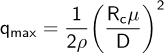
For each sphere, we measured the stagnation pressure at pressure port 3 and the pressure at the aft ports via pressure port 4, which are subtracted to give the pressure difference, delta P. We also measured the test section total pressure, Pt, from pressure port one and the static pressure, Ps, from pressure port two, which are used to determine the test dynamic pressure, q.

Then we can calculate the normalized pressure, which is equal to the pressure difference divided by the dynamic pressure. The air pressure and the airflow temperature were also recorded, enabling the calculation of airflow properties. Recall that there is a slot in the test section, meaning that it is open to ambient air. Therefore, assuming that there is no streamwise pressure gradient in the test section, the absolute value of the local static pressure of the free-stream flow can be used as the ambient air pressure.

The density is obtained using the ideal gas law and the viscosity obtained using Sutherland's formula. Once the air density and viscosity have been determined, we can calculate the Reynolds number. Here we show a plot of the Reynolds number versus the normalized pressure difference, delta P over q.

Using this plot, we can determine the critical Reynolds number for each sphere, since the critical Reynolds number corresponds to a normalized pressure value 1.22. With each critical Reynolds number, we can evaluate the turbulence factor and the effective Reynolds number. The turbulence factor is correlated to the intensity of the turbulence in the wind tunnel.

In summary, we learned how the free-stream turbulence affects testing in a wind tunnel. We then used several smooth spheres to determine the turbulence factor and intensity of the wind tunnel flow and evaluate its quality.

References

- Barlow, Rae and Pope. Low speed wind tunnel testing, John Wiley & Sons, 1999.
- Crawford T.L. and Dobosy R.J. Boundary-Layer Meteorol. 1992. 59; 257-78.
- Eckman R.M., Dobosy R.J., Auble D.L., Strong T.W., and Crawford T.L. J. Atmos. Ocean. Technol. 2007; 24; 994-1007.
. See Tables 1 and 2 for recommended test parameters.