Войдите в систему
Visualization of Flow Past a Bluff Body
Обзор
Source: Ricardo Mejia-Alvarez, Hussam Hikmat Jabbar and Mahmoud N. Abdullatif, Department of Mechanical Engineering, Michigan State University, East Lansing, MI
Owing to the non-linear nature of its governing laws, fluid motion induces complicated flow patterns. Understanding the nature of these patterns has been the subject of intense scrutiny for centuries. Although personal computers and supercomputers are extensively used to deduce fluid flow patterns, their capabilities are still insufficient to determine the exact flow behavior for complex geometries or highly inertial flows (e.g. when momentum dominates over viscous resistance). With this in mind, a multitude of experimental techniques to make flow patterns evident have been developed that can reach flow regimes and geometries inaccessible to theoretical and computational tools.
This demonstration will investigate fluid flow around a bluff body. A bluff body is an object that, due to its shape, causes separated flow over most of its surface. This is in contrast to a streamlined body, like an airfoil, which is aligned in the stream and causes less flow separation. The purpose of this study is to use hydrogen bubbles as a method of visualizing flow patterns. The hydrogen bubbles are produced via electrolysis using a DC power source by submerging its electrodes in the water. Hydrogen bubbles are formed in the negative electrode, which needs to be a very fine wire to ensure that the bubbles remain small and track fluid motion more effectively. This method is suitable for steady and unsteady laminar flows, and is based on the basic flow lines that describe the nature of the flow around objects. [1-3]
This paper focuses on describing the implementation of the technique, including details about the equipment and its installation. Then, the technique is used to demonstrate the use of two of the basics flow lines to characterize the flow around a circular cylinder. These flow lines are used to estimate some important flow parameters like flow velocity and the Reynolds number, and to determine flow patterns.
Процедура
1. To produce a continuous sheet of bubbles:
- Set the equipment according to the electrical diagram shown in Figure 3.
- Fix the positive electrode in the water at the downstream end of the test section (see Figure 4 for reference).
- Fix the negative electrode upstream and near the point of interest to release the bubbles into the stream before the flow reaches the object of study (see Figure 4 for refere
Результаты
Figure 2 shows two representative results of hydrogen bubble visualization of a Von Kármàn vortex street. Figure 2(A) shows an example of a field of streaklines as evidenced by disturbances in the hydrogen bubble sheet. This image is used to extract the diameter of the rod in machine units. Figure 2(B) shows an example of a field of timelines. This image is used to estimate the approaching
Заявка и Краткое содержание
In this study, the usage of hydrogen bubbles was demonstrated to extract qualitative and quantitative information from images of flow around a circular cylinder. The quantitative information extracted from these experiments included the free-stream velocity ( ), vortex-shedding frequency (
 ), Reynolds number (Re), and the Strouhal number (St). In particular, the results for St vs Re exhibited very good agreement with pre
Ссылки
- Zöllner, F. Leonardo da Vinci 1452-1519: sketches and drawings, Taschen, 2004.
- White, F. M. Fluid Mechanics, 7th ed., McGraw-Hill, 2009.
- Adrian, Ronald J., and Jerry Westerweel. Particle Image Velocimetry. Cambridge University Press, 2011.
- Gerrard, J. H., The wakes of cylindrical bluff bodies at low Reynolds number, Phil. Trans. Roy. Soc. (London) Ser. A, Vol. 288, No. 1354, pp. 351-382 (1978)
- Coutanceau, M. and Bouard, R., Experimental determination of the viscous flow in the wake of a circular cylinder in uniform translation. Part 1. Steady flow, J. Fluid Mech., Vol. 79, Part 2, pp. 231-256 (1977)
- Kovásznay, L. S. G., Hot-wire investigation of the wake behind cylinders at low Reynolds numbers, Proc. Roy. Soc. (London) Ser. A, Vol. 198, pp. 174-190 (1949)
- Fey, U., M. König, and H. Eckelmann. A new Strouhal-Reynolds-number relationship for the circular cylinder in the range
 . Physics of Fluids, 10(7):1547, 1998.
 - Maas, H.-G., A. Grün, and D. Papantoniou. Particle Tracking in three dimensional turbulent flows - Part I: Photogrammetric determination of particle coordinates. Experiments in Fluids Vol. 15, pp. 133-146, 1993.
- Malik, N., T. Dracos, and D. Papantoniou Particle Tracking in three dimensional turbulent flows - Part II: Particle tracking. Experiments in Fluids Vol. 15, pp. 279-294, 1993.
- Tropea, C., A.L. Yarin, and J.F. Foss. Springer Handbook of Experimental Fluid Mechanics. Vol. 1. Springer Science & Business Media, 2007.
- Monaghan, J. J., and J. B. Kajtar. Leonardo da Vinci's turbulent tank in two dimensions. European Journal of Mechanics-B/Fluids. 44:1-9, 2014.
- Becker, H.A. Dimensionless parameters: theory and methodology. Wiley, 1976.
 ). This generates a 0 V - 5 V square signal that activates the solid-state relay (closing the circuit) in its high position and opens it in the low position
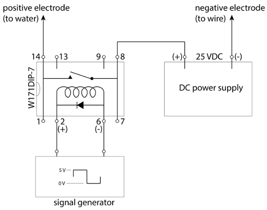
 , using a caliper. Use S.I. units for this measurement (m).
 (points or pixels, depending on format)
 (points or pixels).
 .
. .
.
 m2/s).
 ) measured in step 3.1, the approaching velocity (
 , crossing the reference during a defined period of time
  . A vortex shedding cycle is illustrated in Figure 2(A).
Перейти к...
Видео из этой коллекции:

Now Playing
Visualization of Flow Past a Bluff Body
Mechanical Engineering
11.8K Просмотры
Buoyancy and Drag on Immersed Bodies
Mechanical Engineering
29.9K Просмотры
Stability of Floating Vessels
Mechanical Engineering
22.4K Просмотры
Propulsion and Thrust
Mechanical Engineering
21.6K Просмотры
Piping Networks and Pressure Losses
Mechanical Engineering
58.1K Просмотры
Quenching and Boiling
Mechanical Engineering
7.7K Просмотры
Hydraulic Jumps
Mechanical Engineering
40.9K Просмотры
Heat Exchanger Analysis
Mechanical Engineering
28.0K Просмотры
Introduction to Refrigeration
Mechanical Engineering
24.7K Просмотры
Hot Wire Anemometry
Mechanical Engineering
15.5K Просмотры
Measuring Turbulent Flows
Mechanical Engineering
13.5K Просмотры
Jet Impinging on an Inclined Plate
Mechanical Engineering
10.7K Просмотры
Conservation of Energy Approach to System Analysis
Mechanical Engineering
7.4K Просмотры
Mass Conservation and Flow Rate Measurements
Mechanical Engineering
22.6K Просмотры
Determination of Impingement Forces on a Flat Plate with the Control Volume Method
Mechanical Engineering
26.0K Просмотры

ISSN 2578-7829
Авторские права © 2025 MyJoVE Corporation. Все права защищены
Мы используем файлы cookie для улучшения качества работы на нашем веб-сайте.
Продолжая пользоваться нашим веб-сайтом или нажимая кнопку «Продолжить», вы соглашаетесь принять наши файлы cookie.